
Hello friends of steemit continuing with my publications referring to the science of mathematics today I want to make reference in this post about the normal distribution, which is very important for any statistical process since it allows us to transform the variables into approximate values to the study of certain In this publication, you define your concept, its properties, the variables that define it, as well as the central limit theorem, to complement this information you can see at the end of this post some examples of basic exercises where the standard normal distribution is applied.
Normal distribution
In statistics and probability it is called normal distribution, Gaussian distribution or Gaussian distribution, to one of the probability distributions of continuous variable that most frequently appears statistics and probability theory.
The graph of its density function has a flared shape and is symmetric with respect to a certain statistical parameter. This curve is known as Gaussian bell and is the graph of a Gaussian function.

The green line corresponds to the standard normal distribution
Probability density function
The importance of this distribution lies in the fact that it allows to model numerous natural, social and psychological phenomena. While the mechanisms that underlie much of this type of phenomena are unknown, due to the enormous amount of uncontrollable variables that intervene in them, the use of the normal model can be justified assuming that each observation is obtained as the sum of a few causes independent
In fact, descriptive statistics only allows describing a phenomenon, without any explanation. For the causal explanation, experimental design is necessary, hence the use of statistics in psychology and sociology is known as a correlational method.
The normal distribution is also important because of its relation to the least squares estimation, one of the simplest and oldest estimation methods.
Some examples of variables associated with natural phenomena that follow the normal model are:
- morphological characters of individuals such as stature;
- physiological characters such as the effect of a drug;
- sociological characters such as the consumption of a certain product
by the same group of individuals; - Psychological characters such as the IQ;
- noise level in telecommunications;
- errors made in measuring certain magnitudes;
etc.
The normal distribution also appears in many areas of the statistic itself. For example, the sample distribution of the sample means is approximately normal, when the distribution of the population from which the sample is drawn is not normal. In addition, the normal distribution maximizes the entropy between all the distributions with known mean and variance, which makes it the natural choice of the underlying distribution to a list of summarized data in terms of sample mean and variance. The normal distribution is the most widespread in statistics and many statistical tests are based on a more or less justified "normality" of the random variable under study.
In probability, the normal distribution appears as the limit of several continuous and discrete probability distributions.

Probability distribution function
Formal definition
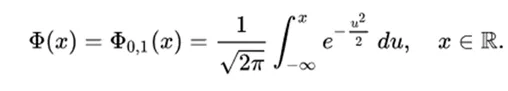
The distribution function of the normal distribution is defined as follows:

Therefore, the distribution function of the standard normal is:
This distribution function can be expressed in terms of a special function called error function in the following way:

and the distribution function itself can, therefore, be expressed as follows:

The complement of the distribution function of the standard normal is denoted with frequency Q (x), and is sometimes referred to simply as a Q function, especially in engineering texts. This represents the probability tail of the Gaussian distribution. Other definitions of the Q function are also occasionally used, which are all simple transformations.
The inverse of the distribution function of the standard normal (quantile function) can be expressed in terms of the inverse of the error function:

and the inverse of the distribution function can, therefore, be expressed as:

This quantile function is sometimes called the probit function. There is no elementary primitive for the probit function. This does not mean merely that it is not known, but that the absence of such a function has been proven. There are several exact methods to approximate the quantile function by the normal distribution (see quantile function).
The values Φ (x) can be approximated very accurately by different methods, such as numerical integration, Taylor series, asymptotic series and continuous fractions.
Strict lower and upper limit for the distribution function
For large values of x the distribution function of the standard normal Φ (x) is very close to  is very close to 0. The elementary limits

in terms of density they are useful.
Using the variable change v = u² / 2, the upper limit is obtained as follows:

Similarly, using the quotient rule,

Generating functions
Moment generating function
The moment generator function is defined as the expectation of e (tX). For a normal distribution, the moment generating function is:

as can be verified by completing the square in the exponent.
Characteristic function
The characteristic function is defined as the expectation of e (itX), where i is the imaginary unit. In this way, the characteristic function is obtained by replacing t by it in the generatrix function of moments. For a normal distribution, the characteristic function is

Properties
Some properties of the normal distribution are the following:

Probability distribution around the mean in a distribution
1 . It is symmetric about its average 
2 . Fashion and the median are both equal to the average,
3 . The turning points of the curve are given for  and
and 
4 . Distribution of probability in an environment of the mean:
1 . in the interval  it is included, approximately, 68.26% of the distribution.
2 . in the interval  there is approximately 95.44% of the distribution.
3 . meanwhile, in the interval  it is comprised, approximately, 99.74% of the distribution. These properties are very useful for the establishment of confidence intervals. On the other hand, the fact that practically the entire distribution is at three standard deviations from the mean justifies the limits of the tables commonly used in the standard normal.
5 . yes  so
so 
6 . yes  are independent normal random variables, then:
Its sum is normally distributed with
 (demonstration). Reciprocally, if two independent random variables have a normally distributed sum, they should be normal (Crámer's Theorem).
- Your difference is normally distributed with

- Your difference is normally distributed with
If the variances of X and Y are equal, then U and V are independent of each other.
The divergence of Kullback-Leibler,

7 .  are independent random variables normally distributed, then:
- Your product X Y follows a distribution with density p, given by

where Ko, is a modified Bessel function of the second type.
- Its quotient follows a Cauchy distribution with
 . In this way the Cauchy distribution is a special type of quotient distribution.
8 . Yes  are standard independent normal variables, then
 follows a χ² distribution with n degrees of freedom.
9 . Yes  are standard independent normal variables, then the sample mean
  and the sample variance
 They are independent. This property characterizes normal distributions and helps explain why the F-test is not robust with respect to non-normality).
General formula of the normal distribution
The Central Limit Theorem
The Central Limit Theorem states that under certain conditions (as they can be independent and identically distributed with finite variance), the sum of a large number of random variables is roughly distributed as a normal one.
The practical importance of the Central Limit Theorem is that the distribution function of the normal one can be used as an approximation of some other distribution functions. For example:
A binomial distribution of parameters n and p is approximately normal for large values of n, and p not too close to 0 or 1 (some books recommend using this approximation only if np and n (1 - p) are both at least 5; a continuity correction should be applied).
The approximate normal has parameters μ = np, σ2 = np (1 - p).A Poisson distribution with parameter λ is approximately normal for large values of λ.
The approximate normal distribution has parameters μ = σ2 = λ.
The accuracy of these approximations depends on the purpose for which they are needed and the rate of convergence to the normal distribution. The typical case is that such approximations are less precise in the tails of the distribution. The Berry-Esséen Theorem provides a general upper limit of the approximation error of the distribution function.
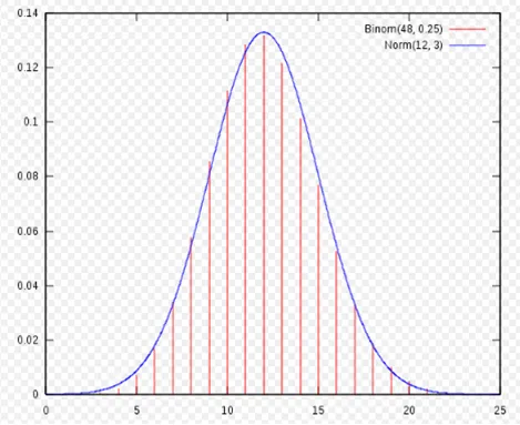
Graph of the distribution function of a normal with μ = 12 and σ = 3, approximating the distribution function of a binomial with n = 48 and p = 1/4.
Below are some examples of exercises where the basic properties of the normal distribution are applied, as well as the general formula.


References
1 . Basic statistics. ITM. 2007. Retrieved on December 12, 2017.
2 . Orrego, Juan José Manzano (2014). PROCUREMENT LOGISTICS. Ediciones Paraninfo, S.A.
3 . Gómez-Chacón, Inés Ma; Català, Claudi Alsina; Raig, Núria Planas; Rodríguez, Joaquim Giménez; Muñoz, Yuly Marsela Vanegas; Sirera, Marta Civil (October 4, 2010). Mathematics education and citizenship. Grao
Four . It is a consequence of the Central Limit Theorem
5 . Abraham de Moivre, "Approximatio ad Summam Terminorum Binomii (a + b) n in Seriem expansi" (printed on November 12, 1733 in London for a private edition). This pamphlet was reprinted in: (1) Richard C. Archibald (1926) "A rare pamphlet of Moivre and some of his discoveries," Isis, vol. 8, pages 671-683; (2) Helen M. Walker, "De Moivre on the law of normal probability" in David Eugene Smith, A Source Book in Mathematics [New York, New York: McGraw-Hill, 1929; reprint: New York, New York: Dover, 1959], vol. 2, pages 566-575; (3) Abraham De Moivre, The Doctrine of Chances (2nd ed.)
6 . Wussing, Hans (March 1998). «Lesson 10». Lessons in the History of Mathematics (1st (Spanish) edition). 21st Century of Spain Editores, S.A. p. 190. "" The normal distribution and its applications to the theory of errors is often associated with the name of Gauss, who discovered it - just as Laplace - independently, but had already been studied by de Moivre. "