
The first chapter (spread over six posts) of my detailed notes on how to contribute to state-of-the-art research in particle physics with Utopian.io and Steem is about to be finalized, this post being the last building block of my introduction to the MadAnalysis 5 framework.
Note that everything beyond the first paragraph may be obscure to anyone who did not read the first 5 posts ;)
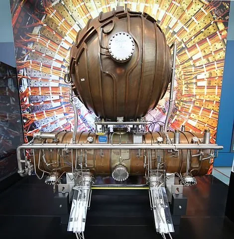
[image credits: Geni (CC BY-SA 4.0)]
This project runs on Steem for a couple of months and aims to offer a chance to developers lying around to help particle physicists in the study of theories extending the Standard Model of particle physics.
All those potential new theories are largely motivated by various important reasons. However, determining how current data from the Large Hadron Collider (the LHC) at CERN constrains this or that model is by far not trivial.
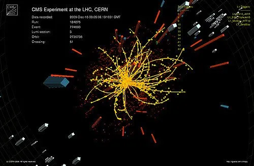
This often requires the simulation of LHC collisions in which signals from given theoretical contexts are generated. One next reanalyzes the LHC results to evaluate data compatibility with those signals. As no hint for any new phenomena has been observed so far, it is clear that one must ensure that any signal stays stealthy.
The above-mentioned tasks require to mimic LHC analysis strategies, and this is where externals developers can enter the game. In this project, I have introduced the MadAnalysis 5 framework, in which C++ implementations of given search LHC strategies have to be achieved.
Providing these C++ codes is where anyone can help!
Of course, there is still a need to detail how to validate those contributions, but this topic is left for after the summer break.
THE MADANALYSIS 5 DATA FORMAT: 5 CLASSES OF OBJECTS
Let me first quickly recapitulate the post important pieces of information provided in the earlier posts, after recalling that installation information can be found in this first post.
In the next two posts (here and there), I introduced the four of the five different classes of objects that could be reconstructed from the information stored in a detector:
- Electrons, that can be accessed through
event.rec()->electrons()in MadAnalysis 5. This consists in a vector ofRecLeptonFormatobjects. - Muons, that can be accessed through
event.rec()->muons()in MadAnalysis 5. This consists in a vector ofRecLeptonFormatobjects. - Photons, that can be accessed through
event.rec()->photons()in MadAnalysis 5. This consists in a vector ofRecPhotonFormatobjects. - Jets, that can be accessed through
event.rec()->jets()in MadAnalysis 5. This consists in sa vector ofRecJetFormatobjects.

[image credits: rawpixel (CC0)]
Surprize surprize: taus are there as well, i.e., the big brothers of the electrons and the muons. It is never to late to introduce them!
They can be accessed as any other guy, through event.rec()->taus()which returns a vector of RecTauFormat objects.
All these different objects have a bunch of properties than can be used when designing an analysis. Those properties are often connected to the tracks left, transversely to the collision axis, by the object in a detector.
One has for instance the object transverse momentum (object.pt()), transverse energy (object.et()) and pseudorapidity (object.eta() or object.abseta() for its absolute value) that somehow describe the motion of the object in the detector.
Finally, analyses are often making use of the energy carried away by some invisible particles. This is in particular crucial for what concerns dark matter, as dark matter is invisible. This ‘missing energy’ can be accessed through
  MALorentzVector pTmiss = event.rec()->MET().momentum();
  double MET = pTmiss.Pt();
that respectively returns a four-vector and a double-precision number.
THE MADANALYSIS 5 DATA FORMAT: OBJECT ISOLATION
[image credits: Todd Barnard (CC BY-SA 2.0)]
Object separation is something primordial to ensure a clean reconstruction in which two specific objects do not leave an overlapping signature in the detector.
The command object1.dr(object2) allows us to evaluate the angular distance between two objects, which is then often imposed to be rather large for quality reasons.
MadAnalysis 5 moreover allows to automatically handle the overlap between jets and electrons through the command PHYSICS->Isol->JetCleaning(MyJets, MyElectrons, 0.2). This returns a cleaned jet collection.
In my last post, I detailed how the CMS experiment was dealing with object isolation. The detector activity within a given angular distance around an object is this time evaluated through
PHYSICS->Isol->eflow->sumIsolation(obj,event.rec(),DR,0.,IsolationEFlow::COMPONENT)
and then constrained. DR indicates here the angular distance around the object obj to consider in the calculations, and COMPONENT has to be TRACK_COMPONENT (charged particles), NEUTRAL_COMPONENT (neutral hadronic particles), PHOTON_COMPONENT (photons) or ALL_COMPONENTS (everything).
SIGNAL REGIONS (ANDMORE WORDS ABOUT HISTOGRAMS)

[image credits: Pixabay (CC0)]
A specific experimental analysis usually focuses on the search for a single signal.
However, it may be possible that such a signal could be probed by several similar analyses, all sharing a common ground and featuring small differences.
One often gather all these ‘sub-analyses’ as a collection of ‘signal regions’ of a single analysis.
As already briefly mentioned in the previous episode, signal regions can easily be declared in the Initialize method of the analysis code by including
  Manager()->AddRegionSelection(“region1”);
  Manager()->AddRegionSelection(“region2”);
  Manager()->AddRegionSelection(“region3”);
  …
Once regions are defined, histograms, introduced in the previous post in the context of a single existing region, can be attached to one or more regions through the commands
  Manager()->AddHisto("histo1",15,0,1200);
  Manager()->AddHisto("histo2",15,0,1200,”region1”);

  std::string reglist[ ] = { "region1", “region2”};
  Manager()->AddHisto("histo3",15,0,1200,reglist);
that must also be included in the Initialize method. The first command attaches a histogram (named histo1) to all existing regions, the second one defines a histogram (named histo2) attached to the region region1, and the third command finally links a third histogram histo3 to the two regions region1 and region2. All histograms are, in this example, made of 15 bins ranging from 0 to 1200.
They are then filled at the level of the Execute method of the analysis code,
Manager()->FillHisto(“histo1”,value)
where value is the weight to be filled in the histogram. This weight is appropriately handled when adding
Manager()->InitializeForNewEvent(event.mc()->weight());
at the beginning of the Execute method.
The digitized version of the histograms can be found in the Output/tth/test_analysis_X/Histograms/histos.saf saf file, where one assumes that the code has been executed on a signal n event named tth.list.
Figures can then be generated by using either the code of @crokkon, of @irelandscape or of @effofex (on GitHub).
IMPLEMENTING A SELECTION STRATEGY

[image credits: Counselling (CC0)]
It is now time to jump with the description of the last ingredients necessary for reimplementing an analysis: cuts (connection with the mower ;) ).
An event selection strategy can be seen as a sequence of criteria (or cuts) deciding whether a given event has to be selected or rejected, the aim being killing the background as much as possible and leaving the signal as untouched as possible.
A cut can hence be seen as a condition which, if realized, leads to the selection of an event. Cuts must first be declared in the Initialize method, in a similar way as for histograms,
 Manager()->AddCut("cutname1”);
 Manager()->AddCut("cutname2","region1");
 Manager()->AddCut("cutname3”,reglist);
The first line introduces a common cut (named cutname1) that is applied to all regions. The second line declares a cut specific to the region region1 and the third line introduces a cut that is common to the two regions region1 and region2.
At the level of the Execute function, the application of a cut has to be implemented as
if(!Manager()->ApplyCut(mycondition, "cutname1")) return true;
where mycondition is a boolean that is true when the event has to be selected. The second argument is simply the name of the cut under consideration. Moreover, cuts have to be applied in the order they have been declared.
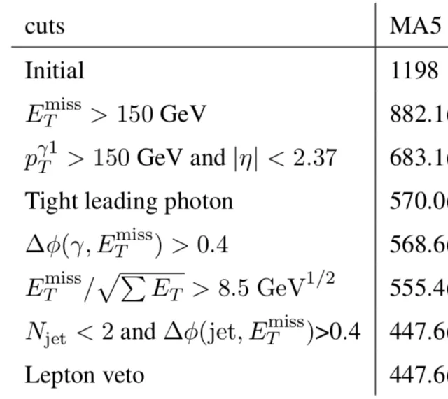
[image credits: arXiv]
The evolution of the number of events surviving the different cuts is what we call a cutflow, an example being shown with the image on the right.
The corresponding information can be found in the Output/tth/test_cms_46/Cutflows directory, tth.list being once again the input file.
In this directory, one SAF file per region is available. For each cut, the line sum of weights is the relevant one to look at for getting the number of events surviving a given cut.
THE EXERCISE
The exercise of the day is pretty simple. We will focus on the earlier CMS search for dark matter and implement the full analysis. We will restart from the piece of codes of the last time and implement the cuts provided in the Section 3 of the CMS article. We will then apply the code to our usual even sample and get a cutflow.
Hint: the azimuthal angle between the missing energy and any object can be computed as object->dphi_0_pi(pTmiss)) with pTmiss being introduced above.
Don’t hesitate to write a post presenting and detailing your code.
- If tagged with utopian-io and blog as the first two tags (and steemstem as a third), the post will be reviewed independently by steemstem and utopian-io.
- If only the steemstem tag is used, the post will be reviewed by steemstem and get utopian-io upvotes through the steemstem trail.
The deadline is Tuesday July 31st, 16:00 UTC.
MORE INFORMATION ON THIS PROJECT
- The idea
- The project roadmap
- Step 1a: implementing electrons, muons and photons
- Step 1b: jets and object properties
- Step 1c: isolation and histograms
- Step 1d: cuts and signal regions (this post)
Participant posts (alphabetical order):
@effofex: histogramming, exercise 1b, madanalysis 5 on windows 10.
@irelandscape: journey through particle physics (1, 2, 2b, 3, 4, 5), exercise 1c and its correction, exercise 1b, exercise 1a.
STEEMSTEM
SteemSTEM is a community-driven project that now runs on Steem for almost 2 years. We seek to build a community of science lovers and to make Steem a better place for Science Technology Engineering and Mathematics (STEM). In particular, we are now actively working in developing a science communication platform on Steem.
More information can be found on the @steemstem blog, in our discord server and in our last project report.